ST-3 Oil Production Data
Andrew Leach
July, 2026
The Alberta Energy Regulator (AER) provides monthly data for oil production in Alberta, including from the oil sands region in a report known as the ST-3. The data are available here, and you can either download the data and analyze it yourself or use the embedded R code below to download all the data.
This page is also an easy introduction for downloading and manipulating data in R. If you’re going to run the R code, you’ll need a few basic set-up elements to get everything to work. I’ve included the code here for your reference.
#packages used
library(tidyverse) #basic set of data wrangling tools from the best part of the R universe
library(readxl) #it does what it says
library(scales) #makes graphs nicer
library(lubridate) #makes dates easier to handle
library(knitr) #using this to make the html document
library(prettydoc) #nice tables in the html doc
library(zoo) #time series data
library(viridis) #color-blind friendly palettes for graphs
library(patchwork) #allows you to combine plots
library(kableExtra) #nice tables in R Markdown
library(curl) #use this for checking internet connections
library(roll) #rolling means
library(ggsci)
library(janitor)
library(httr)

#unit conversions
m3_bbl<-function(x) x*6.2898
bbl_m3<-function(x) x/6.2898


#create tableau palettes

colors_tableau10 <- function()
{
  return(c("#1F77B4", "#FF7F0E", "#2CA02C", "#D62728", "#9467BD", "#8C564B",
           "#E377C2", "#7F7F7F", "#BCBD22", "#17BECF"))
}

colors_tableau10_light <- function()
{
  return(c("#AEC7E8", "#FFBB78", "#98DF8A", "#FF9896", "#C5B0D5", "#C49C94",
           "#F7B6D2", "#C7C7C7", "#DBDB8D", "#9EDAE5"))
}

colors_tableau10_medium <- function()
{
  return(c("#729ECE", "#FF9E4A", "#67BF5C", "#ED665D", "#AD8BC9", "#A8786E",
           "#ED97CA", "#A2A2A2", "#CDCC5D", "#6DCCDA"))
}

download_forbidden_file <- function(url, destfile,refer="https://www.aer.ca/") {
  headers <- c(
    "User-Agent" = "Mozilla/5.0 (Macintosh; Intel Mac OS X 10.14; rv:66.0) Gecko/20100101 Firefox/66.0",
    "Referer" = refer
  )
  r <- GET(
    url,
    add_headers(.headers = headers)
  )
  stop_for_status(r)
  writeBin(
    content(r, "raw"),
    destfile
  )
  invisible(destfile)
}
Download the Data
Once you’ve got the preliminaries of the code, downloading the data is fairly easy. Each of the data files are stored by year, with the exception of the current year which has a different naming convention. The first step is to access the data (click on the code button to see how to do things in R if you’re interested). The code also includes some fixes for names of projects which are not consistent in the data. This is basically a trial and error process to find broken data series.
#I'm going to make a function here so that I can specify whether I want to download all/none/new

st_3_online<-function(download="none"){
   #every year is xlss file which makes it easy
#specify the rows we're going to want
#download="none"
  #keep_rows<-c("Crude Oil Light",  "Crude Oil Medium",
#             "Crude Oil Heavy","Crude Oil Ultra Heavy","Total Conventional Oil Production","Crude Oil Ultra-Heavy",
#             "Condensate Production","In Situ Production","Mined Production",
#             "Non-Upgraded Total","Upgraded Production","Total Oil Sands Production",
#             "Total Production","Nonupgraded Total")
#use a list to store each of the data sets we're going to download
data_store <- list()
years<-seq(2010,2016)
i<-1
  filename<-paste("Oil_2010-2016.xlsx",sep="")
  if(tolower(download)=="all")#if you chose to download the old data. correct case errors in case someone sends "ALL"
        if(has_internet()) #if you're connected, go get the file
          if(!file.exists(filename))
          download.file(paste("https://www.aer.ca/documents/sts/st3/",filename,sep=""),filename,mode="wb")
#year<-2010 #testing
for(year in years){ #loop over 2010-2016, but the data are stored in different sheets
  production_data <- read_excel(filename, sheet = as.character(year), skip = 4)
  #the sheets are a bit of a mess, so we need to clean them up
  names(production_data)[1]<-"product" #name column 1
  # the %>% or pipeline is basically a  "pass to" command
  # start with production data, pass to select and remove cols 2 and 15, pass to filter and keep and rows with
  # the names in the keep_rows object we created above
  production_data<-production_data %>% select(-2,-15)%>% #%>% filter(product %in% keep_rows)
  filter(!is.na(product),!is.na(Jan))%>%
  mutate(across(-1, as.numeric))
  #rename the column with the annual data s (grep is a search function that, in this case, is looking for
  #whatever year we're processing and it will name the column annual
  names(production_data)[grep(as.character(year),names(production_data))]<-"annual"
  #assign the year to whatver year we're processing
  production_data$year<-year
  # create a long-form data set that will have product, annual level for that product, the year we're processing, and     #the monthly data
  production_data<-production_data %>% pivot_longer(cols=-c("product","annual","year"),
                                            names_to="month",values_to = "production")
  #store those data in a node in the list
  data_store[[i]]<-production_data
  #step your list counter one unit
  i<-i+1
  }
  #let's get 2017-2020 data - same process, but they are in seperate files
  #https://static.aer.ca/prd/documents/sts/st3/ST3_2021-12_Oil.xlsx
  years<-seq(2017,2025)
  #year<-2023
  for(year in years){ #loop over 2017-2020
    filename<-paste("Oil_",year,".xlsx",sep="") #use paste to put the year into the filename
    if(year==2025)
        filename<-"Oil_2025.xlsx"
    if(year==2024)
        filename<-"ST3_Oil_2024.xlsx"
    if(year==2023)
        filename<-"ST3_2023-12_Oil.xlsx"
    if(year==2022)
        filename<-"ST3_2022-12_Oil.xlsx"
    if(year==2021)
        filename<-"ST3_2021-12_Oil.xlsx"
    if(tolower(download)=="all")#if you chose to download the old data. correct case errors in case someone sends "ALL"
        if(has_internet()) #if you're connected, go get the file
          if(!file.exists(filename))
            if(year!=2024)
            download_forbidden_file(paste("https://www.aer.ca/documents/sts/st3/",filename,sep=""),filename)
    if(has_internet()) #if you're connected, go get the file
          if(!file.exists(filename))
            if(year==2024)
            download_forbidden_file("https://www.aer.ca/2025-02/ST3_Oil_2024.xlsx",filename,mode="wb")
      if(has_internet()) #if you're connected, go get the file
          if(!file.exists(filename))
            if(year==2025)
            download_forbidden_file("https://www.aer.ca/prd/documents/sts/st3/Oil_2025.xlsx",filename)
    production_data <- read_excel(filename, sheet = "Data", skip = 4)
    names(production_data)[1]<-"product"
    production_data<-production_data %>% select(-2,-15) %>% filter(!is.na(product),!is.na(Jan))%>%
  mutate(across(-1, as.numeric))
    names(production_data)[grep(as.character(year),names(production_data))]<-"annual"
    production_data$year<-year
    production_data<-production_data %>% pivot_longer(cols=-c("product","annual","year"),
                                              names_to="month",values_to = "production")
    data_store[[i]]<-production_data


    i<-i+1
  }
  #Most recent data are stored as "current"
  filename<-"Oil_current.xlsx"
  #download.file("https://www.aer.ca/documents/sts/st3/Oil_current.xlsx",destfile=filename,mode="wb")
url<-"https://www.aer.ca/documents/sts/st3/Oil_current.xlsx"

needs_refresh <- !file.exists(filename) ||
  difftime(Sys.time(), file.info(filename)$mtime, units = "hours") > 24
if(needs_refresh)
  download_forbidden_file(url,  filename,refer="https://www.aer.ca/")

# then manually trigger download or extract via browser context
  #check for interne
#  if(has_internet()) #if you're connected, go get the file
#      download.file("https://www.aer.ca/documents/sts/st3/Oil_current.pdf",filename,mode="wb")
      #download.file(paste("https://www.aer.ca/documents/sts/st3/",filename,sep=""),filename,mode="wb")
  production_data <- read_excel(filename, sheet = "Data", skip = 4)
  year<-2026
  names(production_data)[1]<-"product"
  production_data<-production_data %>% select(-2,-15) %>% filter(!is.na(product),!is.na(Jan))%>%
  mutate(across(-1, as.numeric))
  names(production_data)[grep(as.character(year),names(production_data))]<-"annual"
  production_data$year<-year
  production_data<-production_data %>% pivot_longer(cols=-c("product","annual","year"),
                                              names_to="month",values_to = "production")
  production_data<-production_data %>% filter(production!=0)#keep only non-zero production
  data_store[[i]]<-production_data

  #now, stack all the elements stored in your list of data into a data frame
  all_production<-do.call(rbind,data_store)
  #now, we'll manipulate the data. mutate is adding a column based on a calculation
  #so, all_production is all_prodcution passed to mutate, where the production variable is set to numeric
  #and we format the dates using ymd since that's the format in the spreadsheet
  # (remember, the lubridate package makes dates easy)
  all_production<-all_production %>% mutate(production=as.numeric(production),
                                            date=ymd(paste(year,as.character(month),1,sep="-")))

  save(all_production,file = "st3_oil.rdata")
  #next part is working with factors. Factors basically store data as a numeric code or level (1,2,3,4) and a
  #set of labels attached to the levels

  #take all_production,and pass to mutate, change the column product to a factor
  all_production <-all_production %>% mutate(product=as_factor(product)) %>%
                                      #and now we're going to re-code some of the labels so that we make them common                                          #across the data we loaded
                                      mutate(
                                             product=fct_recode(product,
                                                                "In Situ Bitumen"="In Situ Production",
                                                                "Mined Bitumen"="Mined Production",
                                                                "Non-Upgraded Bitumen"="Non-Upgraded Total",
                                                                "Non-Upgraded Bitumen"="Nonupgraded Total",
                                                                "Synthetic Crude"="Upgraded Production",
                                                                "Conventional Oil"="Total Crude Oil Production",
                                                                "Conventional Oil"="Total Conventional Oil Production",
                                                                "Total"="Total Production",
                                                                "Total Oil Sands"="Total Oil Sands Production",
                                                                "Condensate"="Condensate Production"
                                                                ),
                                             #and we're going to sort them so that mined bitumen is last
                                             product=fct_relevel(product,"Mined Bitumen",after=5))
 #last, we're going to collapse factors into on common level, so light and medium go into light, heavy and ultra-heavy
 #are classified as heavy

  all_production <-all_production %>% mutate(product=fct_collapse(product,
                        "Conventional Light Oil" = c("Crude Oil Light","Crude Oil Medium"),
                        "Conventional Heavy Oil"= c("Crude Oil Heavy","Crude Oil Ultra Heavy")
                        )) %>%
    #now, because for some rows we'll now have 2 entries for production from conventional light oil, for example,
    # in a month, we have to collapse them
    #group your data by product, year, month, and date
                    group_by(product,year,month,date)%>%
    #and combined the monthly and annual production from all prducts with the same label by summing them
                          summarize(production=sum(production),annual=sum(as.numeric(annual))) %>%
                          ungroup()

  #last thing - we'll use zoo to create some time series descriptives
  #add year and quarter
  all_production <-all_production %>% mutate(year=year(date), quarter=quarter(date))%>%
  #add rolling quarterly and annual data and lags
    group_by(product)%>% arrange(date)%>% mutate(
      roll_4m=roll_mean(production,4),
      roll_12m=roll_sum(production,12),
      growth_12m=(roll_12m-lag(roll_12m,12))/lag(roll_12m,12),
      lag12_raw=(production-lag(production,12))/lag(production,12),
      lag12_roll=(roll_4m-lag(roll_4m,12))/lag(roll_4m,12))
  #and that's it - you've made a data set of Alberta oil production for the last decade

  all_production # the last thing the function does is what it returns. We want it to return the data set

}

all_production<-st_3_online(download = "none") #call the function we just made to get the data
save(all_production,file = "st3_oil.rdata")
#create an annual data set using group_by and summarize

  annual<-all_production %>%
    mutate(days=days_in_month(date))%>%
    group_by(year,product) %>% summarise(production=sum(production),
          days=sum(days))%>%
    arrange(year)%>% group_by(product)%>%
    mutate(yoy_growth=round((production-lag(production,1))/lag(production,1)*100,2))

#create an annual data set using group_by and summarize

#same for a quarterly data_set

  quarterly<-all_production %>%
    mutate(days=days_in_month(date))%>%
    group_by(year,quarter,product) %>% summarise(production=mean(production),days=sum(days))
  quarterly <-quarterly %>%arrange(year,quarter)%>% group_by(product)%>%
    mutate(q_lasty=round((production-lag(production,4))/lag(production,4)*100,2))
With the data downloaded and compiled into a single file, with annual and quarterly subfiles, we can graph some data.
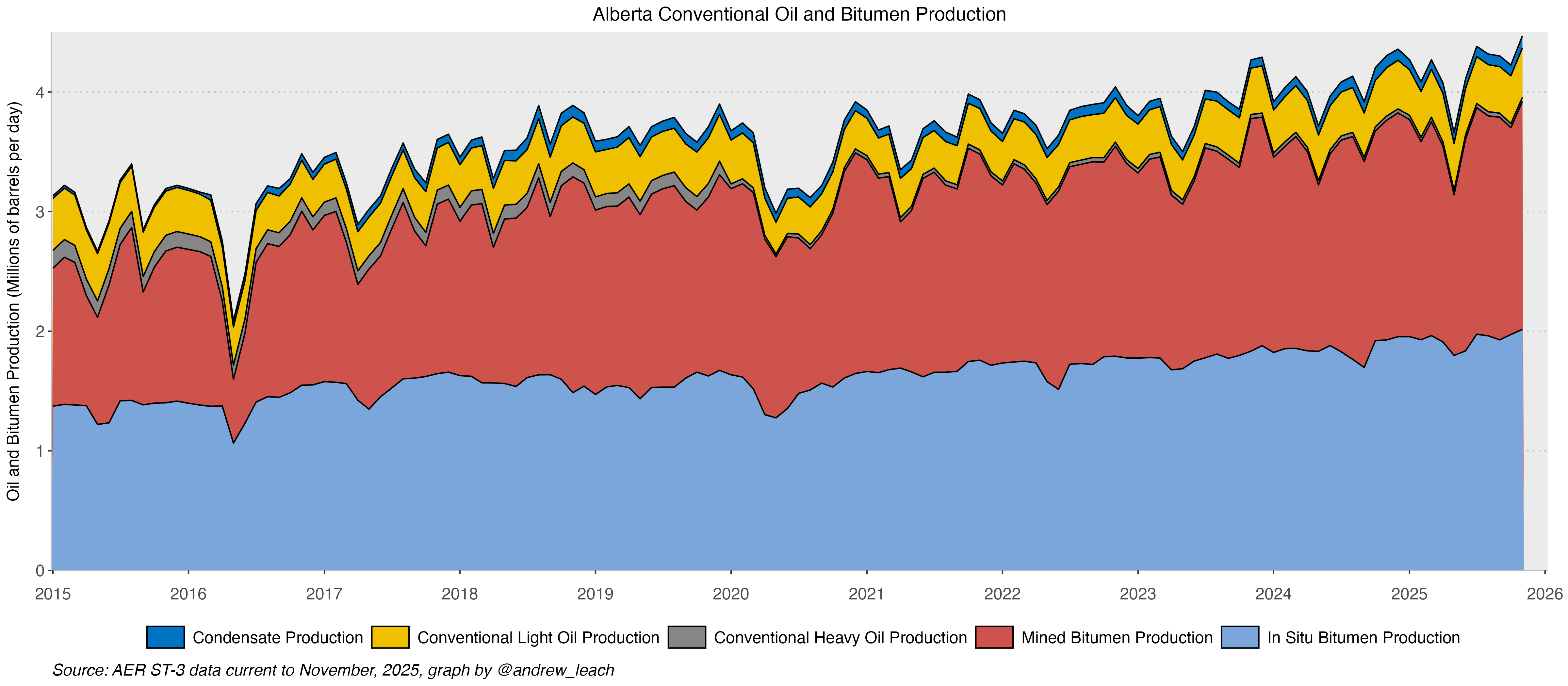
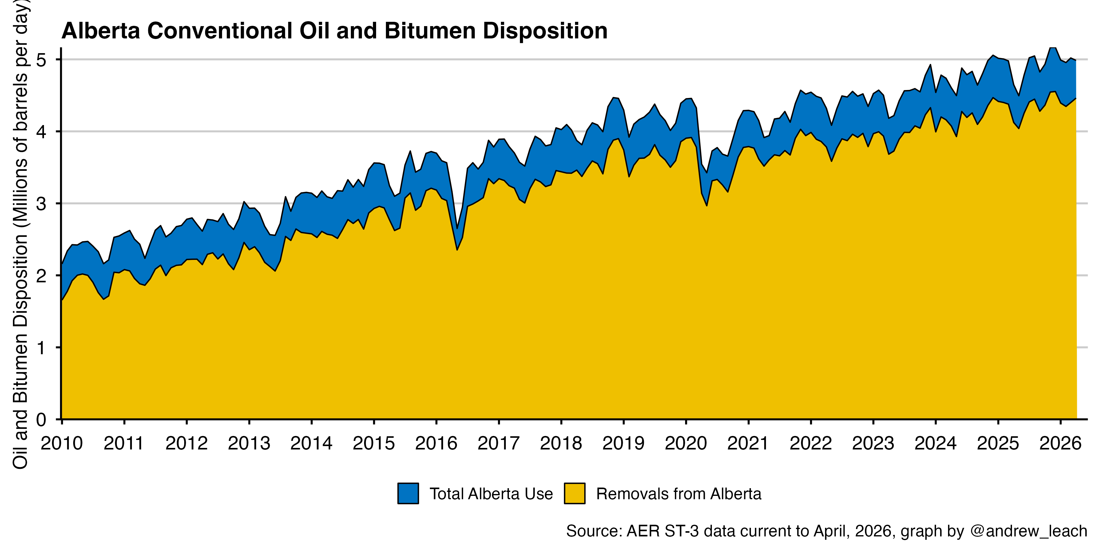
dispo<-
ggplot(filter(all_production,product%in%c("Total Alberta Use","Removals from Alberta")))+
geom_area(aes(date,m3_bbl(production)/days_in_month(date)/10^6,group=product,fill=product),color="black", size=0.5)+
scale_fill_manual("",values = pal_jco()(10),guide = "legend")+
#scale_fill_viridis("",discrete = T,option="F",direction = -1,end = .9)+
scale_x_date(date_breaks = "1 year",date_labels = "%Y",expand = c(0,0))+
scale_y_continuous(expand = c(0,0),breaks=pretty_breaks())+
#scale_colour_manual("",values=my_palette,guide = "legend")+
guides(fill=guide_legend(nrow=1))+
expand_limits(y=4.5)+
expand_limits(x=Sys.Date())+
theme_irpp(base_size = 16)+
rotate_x()+
labs(y="Oil and Bitumen Disposition (Millions of barrels per day)",x=NULL,
title="Alberta Conventional Oil and Bitumen Disposition",
#subtitle="For Operators with Production above 25k bbl/d",
caption=paste("Source: AER ST-3 data current to ",format.Date(max(all_production$date),format = "%B, %Y") ,", graph by @andrew_leach",sep=""))
#dispo
ggsave(plot=dispo,filename = "st3_dispo.png",width=11,height=6.5,dpi=300,bg="white")
graph_data<-c("Conventional Light Oil","Conventional Heavy Oil","Condensate",
"In Situ Bitumen","Mined Bitumen")
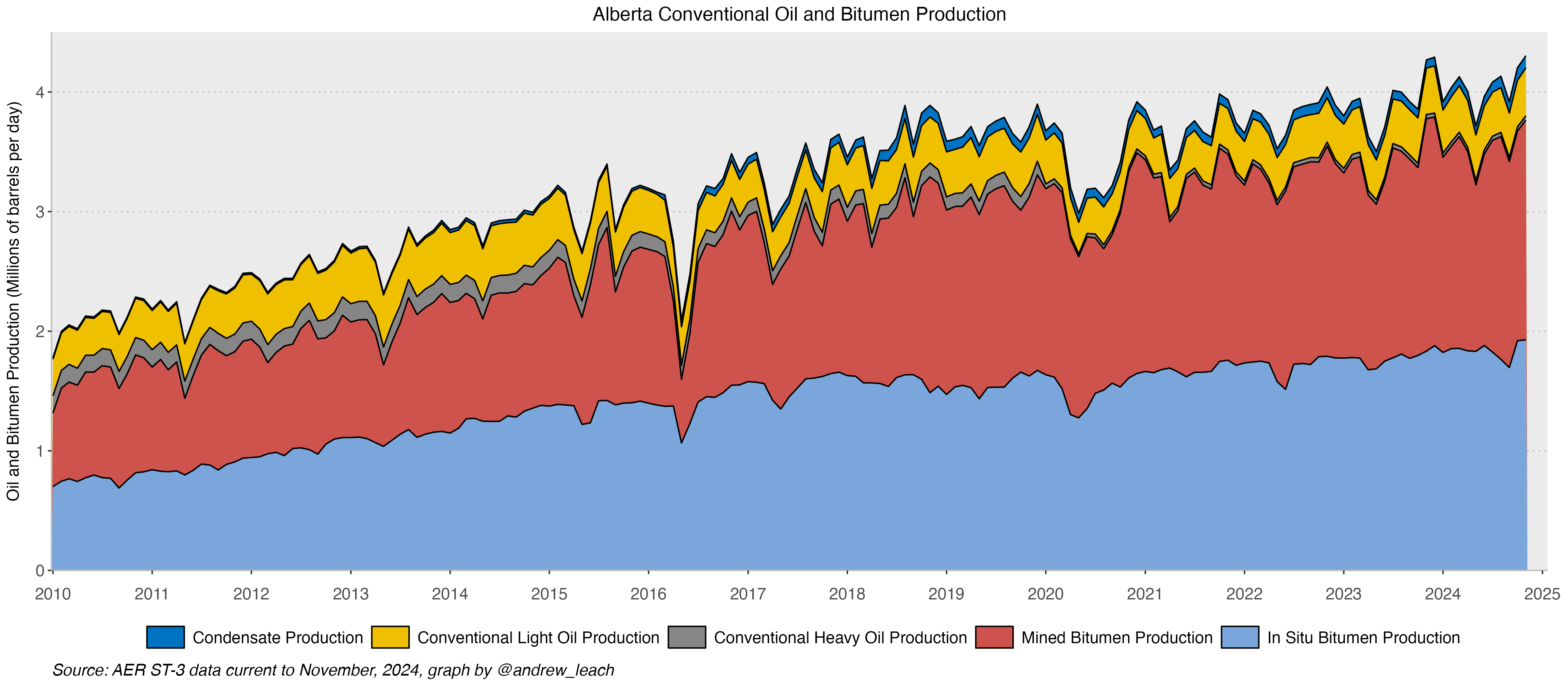
all_crude<-ggplot(filter(all_production,product%in%graph_data)%>%
mutate(product=fct_relevel(product,"Condensate")))+
geom_area(aes(date,m3_bbl(production)/days_in_month(date)/10^6,group=product,fill=product),color="black", size=0.5)+
scale_fill_manual("",values = pal_jco()(10),guide = "legend")+
#scale_fill_viridis("",discrete = T,option="F",direction = -1,end = .9)+
scale_x_date(date_breaks = "1 year",date_labels = "%Y",expand = c(0,0))+
scale_y_continuous(expand = c(0,0),breaks=pretty_breaks())+
#scale_colour_manual("",values=my_palette,guide = "legend")+
guides(fill=guide_legend(nrow=1))+
expand_limits(y=4.5)+
expand_limits(x=Sys.Date())+
theme_irpp(base_size = 16)+
labs(y="Oil and Bitumen Production (Millions of barrels per day)",x=NULL,
title="Alberta Conventional Oil and Bitumen Production",
#subtitle="For Operators with Production above 25k bbl/d",
caption=paste("Source: AER ST-3 data current to ",format.Date(max(all_production$date),format = "%B, %Y") ,", graph by @andrew_leach",sep=""))
#all_crude
#if you want to create a png in normal code, use this
#ggsave(all_crude,"oil_prod.png",width=12,height=6)
all_crude_short<-ggplot(filter(all_production,year>=2015,product%in%graph_data)%>%
mutate(product=fct_relevel(product,"Condensate")))+
geom_area(aes(date,m3_bbl(production)/days_in_month(date)/10^6,group=product,fill=product),color="black", size=0.5)+
scale_fill_manual("",values = pal_jco()(10),guide = "legend")+
#scale_fill_viridis("",discrete = T,option="F",direction = -1,end = .9)+
scale_x_date(date_breaks = "1 year",date_labels = "%Y",expand = c(0,0))+
scale_y_continuous(expand = c(0,0),breaks=pretty_breaks())+
#scale_colour_manual("",values=my_palette,guide = "legend")+
guides(fill=guide_legend(nrow=1))+
expand_limits(y=4.5)+
expand_limits(x=Sys.Date())+
theme_irpp(base_size = 16)+
labs(y="Oil and Bitumen Production (Millions of barrels per day)",x=NULL,
title="Alberta Conventional Oil and Bitumen Production",
#subtitle="For Operators with Production above 25k bbl/d",
caption=paste("Source: AER ST-3 data current to ",format.Date(max(all_production$date),format = "%B, %Y") ,", graph by @andrew_leach",sep=""))
#all_crude_short
all_crude_weekly<-ggplot(filter(all_production,product%in%graph_data))+
geom_area(aes(date,6.2898*(production)/days_in_month(date)/10^6,group=product,fill=product))+
scale_fill_manual("",values = colors_tableau10(),guide = "legend")+
scale_x_date(date_breaks = "6 months",date_labels = "%b\n%Y",expand = c(0,0))+
scale_y_continuous(expand = c(0,0),breaks=pretty_breaks())+
#scale_colour_manual("",values=my_palette,guide = "legend")+
guides(fill=guide_legend(nrow=2))+
scale_fill_manual(NULL,values=colors_ua10())+
scale_x_date(date_breaks = "1 year", date_labels = "%b\n%Y",expand=c(0,0))+
scale_y_continuous(expand = c(0, 0)) +
guides(fill=guide_legend(nrow=2))+
labs(y="Oil and Bitumen Production (Millions of barrels per day)",x=NULL,
title="Alberta Conventional Oil and Bitumen Production",
#subtitle="For Operators with Production above 25k bbl/d",
caption=paste("Source: AER ST-3 data current to ",format.Date(max(all_production$date),format = "%B, %Y") ,", graph by @andrew_leach",sep=""))+
theme_irpp(base_size = 16)
#if you want to create a png in normal code, use this
#save(all_crude_weekly,file="../weekly_charts/st3_prod.gph")
#ggsave(all_crude_weekly,file="../weekly_charts/st3_prod.gph")
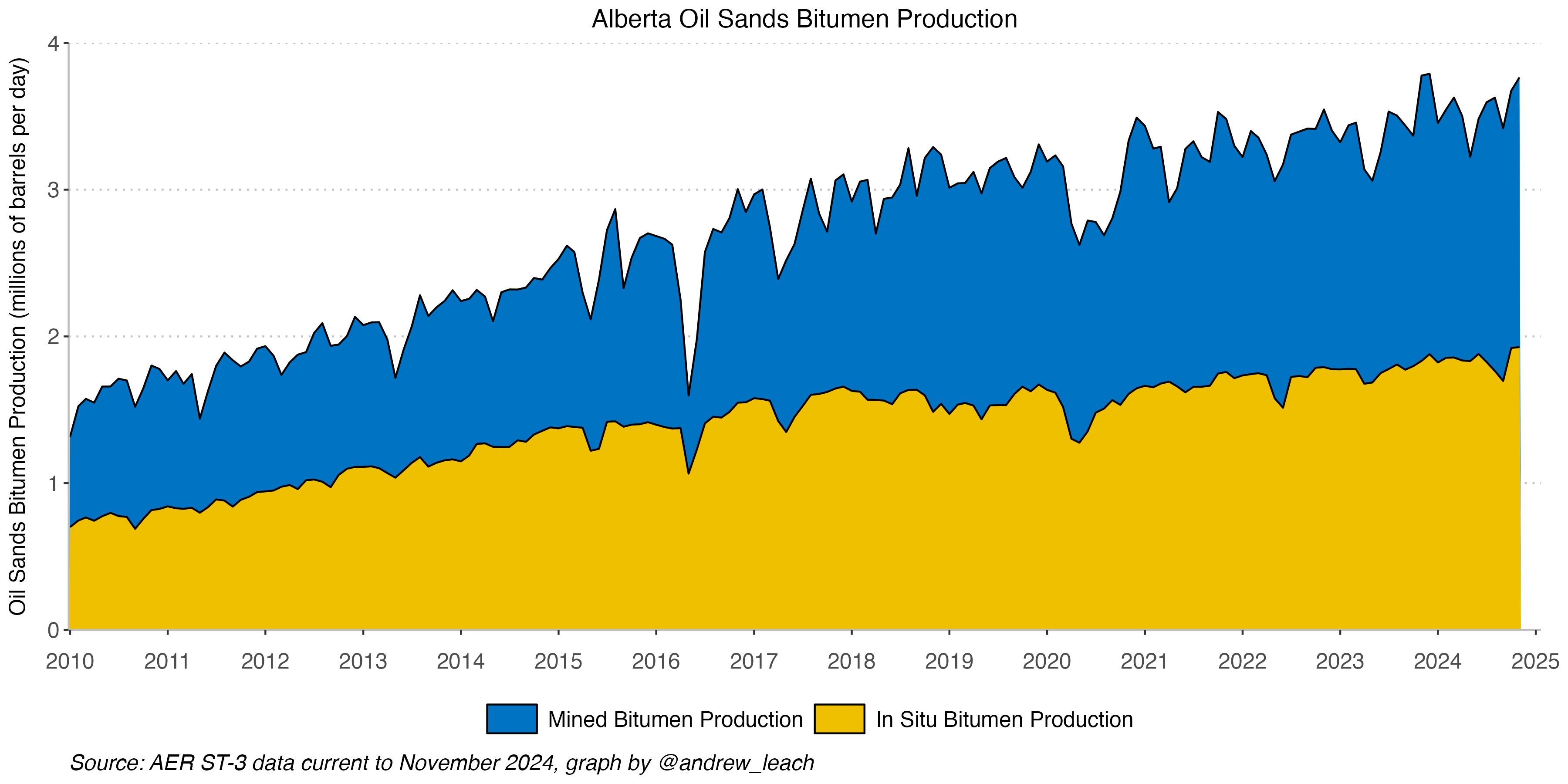
oil_sands<-
ggplot(filter(all_production,product%in%graph_data,product!="Total Conventional Oil",product!="Conventional Heavy Oil",product!="Conventional Light Oil",product!="Condensate"))+
geom_area(aes(date,m3_bbl(production)/days_in_month(date)/10^6,group=product,fill=product),color="black",size=0.5)+
#scale_fill_viridis("",discrete = T,option="A",direction = -1,end = .9)+
scale_fill_manual("",values = pal_jco()(2),guide = "legend")+
scale_x_date(date_breaks = "1 year",date_labels = "%Y",,expand = c(0,0))+
scale_y_continuous(expand = c(0,0),breaks=pretty_breaks())+
expand_limits(y=4)+
#scale_colour_manual("",values=my_palette,guide = "legend")+
#guides(fill=FALSE,colour=FALSE)+
expand_limits(x=Sys.Date())+
guides(fill=guide_legend(nrow=1))+
theme_irpp(base_size = 16)+
labs(y="Oil Sands Bitumen Production (millions of barrels per day)",x=NULL,
title="Alberta Oil Sands Bitumen Production",
caption=paste("Source: AER ST-3 data current to ",format.Date(max(all_production$date),format = "%B %Y") ,", graph by @andrew_leach",sep=""))
#oil_sands
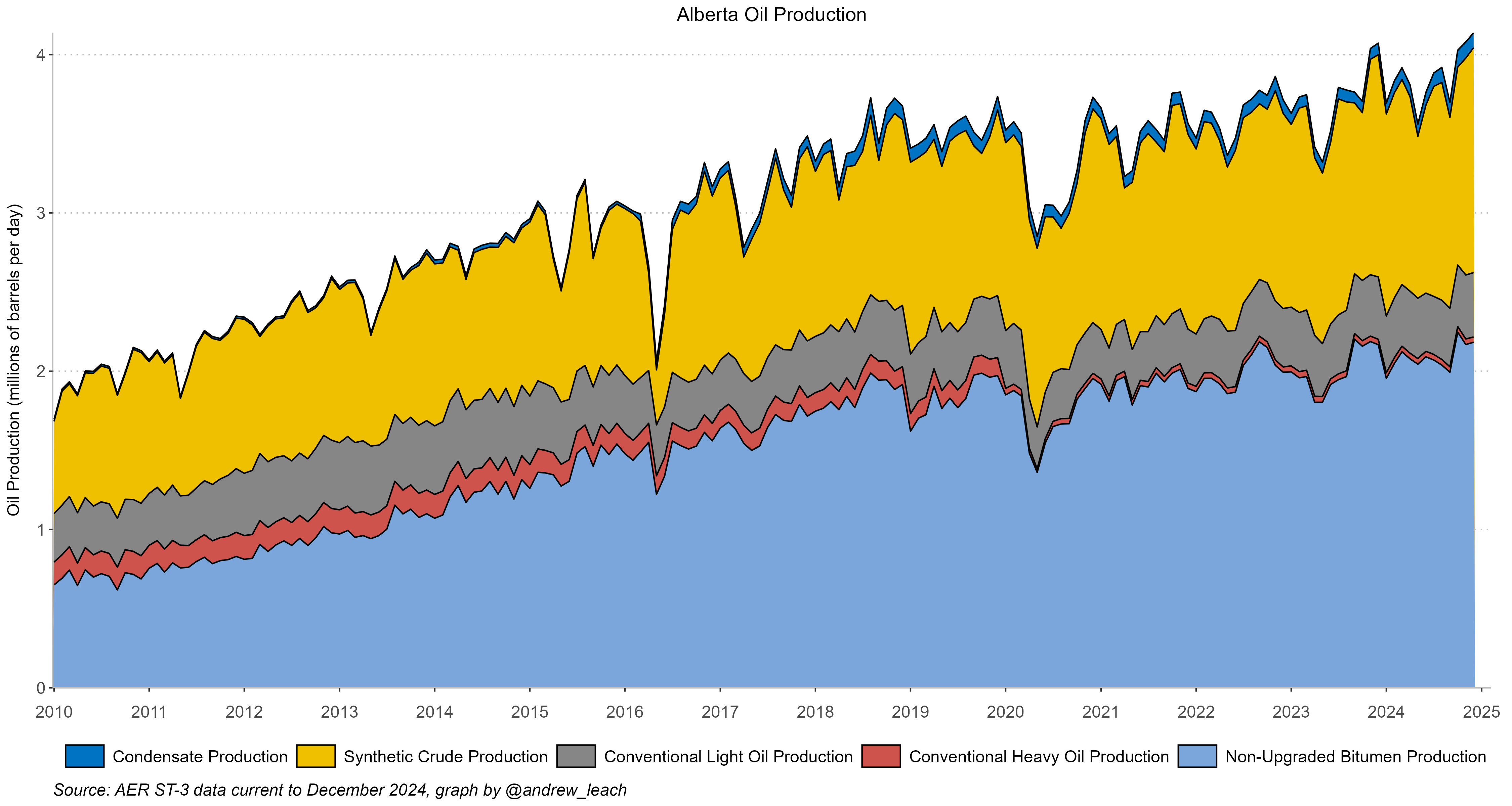
upgraded<-
all_production%>%filter(product%in%c("Non-Upgraded Bitumen","Conventional Heavy Oil","Conventional Light Oil","Synthetic Crude","Condensate"))%>%
mutate(product=factor(product,levels =c("Non-Upgraded Bitumen","Conventional Heavy Oil","Conventional Light Oil","Synthetic Crude","Condensate")),
product=fct_rev(product)
)%>%
ggplot()+
geom_area(aes(date,m3_bbl(production)/days_in_month(date)/10^6,group=product,fill=product),color="black",size=0.5)+
#scale_fill_viridis("",discrete = T,option="A",direction = -1,end = .9)+
scale_fill_manual("",values = pal_jco()(5),guide = "legend")+
scale_x_date(date_breaks = "1 year",date_labels = "%Y",,expand = c(0,0))+
scale_y_continuous(expand = c(0,0),breaks=pretty_breaks())+
expand_limits(y=4)+
#scale_colour_manual("",values=my_palette,guide = "legend")+
#guides(fill=FALSE,colour=FALSE)+
expand_limits(x=Sys.Date())+
guides(fill=guide_legend(nrow=1))+
theme_irpp(base_size = 16)+
labs(y="Oil Production (millions of barrels per day)",x=NULL,
title="Alberta Oil Production",
caption=paste("Source: AER ST-3 data current to ",format.Date(max(all_production$date),format = "%B %Y") ,", graph by @andrew_leach",sep=""))
#if you want to create a png in normal code, use this
ggsave(plot=upgraded,filename = "st3_oil_sands_upg.png",width=15,height=8,dpi=300,bg="white")
oil_sands_plain<-ggplot(filter(all_production,product%in%graph_data,product!="Total Conventional Oil",product!="Conventional Heavy Oil",product!="Conventional Light Oil",product!="Condensate"))+
geom_area(aes(date,m3_bbl(production)/days_in_month(date)/10^6,group=product,fill=product),color="black",size=0.5)+
scale_fill_manual("",values = grey.colors(n=3,end=0.85,start = 0.3),guide = "legend")+
scale_x_date(date_breaks = "1 year",date_labels = "%b\n%Y",,expand = c(0,0))+
scale_y_continuous(expand = c(0,0),breaks=pretty_breaks())+
expand_limits(y=4)+
expand_limits(x=Sys.Date(),y=4.4)+
guides(fill=guide_legend(nrow=1))+
theme_irpp(base_size = 16)+
labs(y="Oil Sands Bitumen Production (millions of barrels per day)",x=NULL)
#title="Alberta Oil Sands Bitumen Production",
#caption=paste("Source: AER ST-3 data current to ",format.Date(max(all_production$date),format = "%B %Y") ,", graph #by @andrew_leach",sep=""))
#if you want to create a png in normal code, use this
ggsave(plot=oil_sands,filename = "st3_oil_sands_prod.png",width=12,height=6,dpi=300,bg="white")

All production
all_crude_short
ggsave(plot=all_crude_short,filename = "st3_oil_prod_short.png",width=16,height=7,dpi=300,bg="white")Click here for high-resolution image
all_crude
#save(all_crude,file="../ab_budget/st3_prod.gph")

ggsave(plot=all_crude,filename = "st3_oil_prod.png",width=16,height=7,dpi=300,bg="white")
Click here for high-resolution image
upgraded

Recent Production (mmbbl/d)
  all_production%>%filter(product%in%c("Conventional Light Oil","Conventional Heavy Oil","Mined Bitumen","In Situ Bitumen","Total Oil Sands","Total"),date>=max(date)-years(1)) %>%
  select(product,date,production)%>%
  mutate(production=m3_bbl(production)/10^6/days_in_month(date),
         product=gsub(" Production","",product))%>%
  pivot_wider(names_from=product,values_from = production)%>%
  mutate(date=format(date,"%b %Y")
         )%>%rename(Date=date)%>%
   kbl(escape = FALSE,table.attr = "style='width:100%;'") %>%
    kable_styling(fixed_thead = T,bootstrap_options = c("hover", "condensed","responsive"),full_width = T)%>%
  #scroll_box(width = "1000px", height = "600px")%>%
  column_spec(1, extra_css = "white-space: nowrap;") %>%
      I()
## Warning in readRDS(responseFile): invalid or incomplete compressed data| Date | Conventional Light Oil | Conventional Heavy Oil | Mined Bitumen | In Situ Bitumen | Total Oil Sands | Total |
|---|---|---|---|---|---|---|
| May 2025 | 0.393 | 0.036 | 1.34 | 1.80 | 2.96 | 3.61 |
| Jun 2025 | 0.388 | 0.035 | 1.77 | 1.84 | 3.42 | 4.06 |
| Jul 2025 | 0.392 | 0.035 | 1.89 | 1.98 | 3.67 | 4.31 |
| Aug 2025 | 0.392 | 0.035 | 1.84 | 1.96 | 3.58 | 4.23 |
| Sep 2025 | 0.386 | 0.035 | 1.86 | 1.93 | 3.57 | 4.21 |
| Oct 2025 | 0.396 | 0.036 | 1.73 | 1.97 | 3.48 | 4.14 |
| Nov 2025 | 0.410 | 0.036 | 1.91 | 2.02 | 3.72 | 4.40 |
| Dec 2025 | 0.397 | 0.035 | 1.96 | 1.99 | 3.75 | 4.40 |
| Jan 2026 | 0.392 | 0.036 | 1.77 | 2.01 | 3.55 | 4.21 |
| Feb 2026 | 0.400 | 0.035 | 1.67 | 2.02 | 3.49 | 4.15 |
| Mar 2026 | 0.411 | 0.034 | 1.70 | 2.02 | 3.50 | 4.17 |
| Apr 2026 | 0.414 | 0.034 | 1.73 | 1.97 | 3.47 | 4.15 |
| May 2026 | 0.405 | 0.032 | 1.67 | 1.86 | 3.33 | 3.99 |
Annual Production (mmbbl/d)
  annual%>%filter(product%in%c("Conventional Light Oil","Conventional Heavy Oil","Mined Bitumen","In Situ Bitumen","Total Oil Sands","Total")) %>%
  mutate(production=m3_bbl(production)/10^6/days,
         product=gsub(" Production","",product))%>%select(-yoy_growth)%>%pivot_wider(names_from=product,values_from = production)%>%
  rename(Year=year)%>%
  select(-days)%>%
  mutate(Year=ifelse(Year==last(Year),paste(Year,"(to date)"),Year))%>%
   kbl(escape = FALSE,table.attr = "style='width:100%;'") %>%
    kable_styling(fixed_thead = T,bootstrap_options = c("hover", "condensed","responsive"),full_width = T)%>%
  #scroll_box(width = "1000px", height = "600px")%>%
  column_spec(1, extra_css = "white-space: nowrap;") %>%
I() | Year | Conventional Light Oil | Conventional Heavy Oil | Mined Bitumen | In Situ Bitumen | Total Oil Sands | Total |
|---|---|---|---|---|---|---|
| 2010 | 0.316 | 0.144 | 0.857 | 0.763 | 1.49 | 1.97 |
| 2011 | 0.347 | 0.144 | 0.893 | 0.859 | 1.64 | 2.14 |
| 2012 | 0.407 | 0.149 | 0.930 | 1.009 | 1.82 | 2.39 |
| 2013 | 0.431 | 0.151 | 0.976 | 1.117 | 1.96 | 2.56 |
| 2014 | 0.439 | 0.151 | 1.038 | 1.272 | 2.17 | 2.79 |
| 2015 | 0.392 | 0.137 | 1.162 | 1.368 | 2.38 | 2.93 |
| 2016 | 0.326 | 0.118 | 1.147 | 1.393 | 2.41 | 2.91 |
| 2017 | 0.332 | 0.114 | 1.275 | 1.550 | 2.67 | 3.18 |
| 2018 | 0.372 | 0.117 | 1.472 | 1.583 | 2.91 | 3.49 |
| 2019 | 0.375 | 0.112 | 1.551 | 1.556 | 2.95 | 3.52 |
| 2020 | 0.323 | 0.033 | 1.483 | 1.504 | 2.83 | 3.33 |
| 2021 | 0.324 | 0.034 | 1.592 | 1.680 | 3.10 | 3.61 |
| 2022 | 0.359 | 0.035 | 1.617 | 1.715 | 3.16 | 3.73 |
| 2023 | 0.374 | 0.037 | 1.647 | 1.776 | 3.23 | 3.82 |
| 2024 | 0.382 | 0.035 | 1.714 | 1.848 | 3.36 | 3.98 |
| 2025 | 0.394 | 0.036 | 1.767 | 1.936 | 3.50 | 4.15 |
| 2026 (to date) | 0.404 | 0.034 | 1.709 | 1.975 | 3.47 | 4.13 |
Annual Production History from ST-98 (mmbbl/d)
#get longer history files from ST98


#download.file("https://www.aer.ca/documents/sts/st98/2025/st98-2025-executive-summary-data.xlsx",mode="wb",dest="st98_exec.xlsx")
energy_supply<-read_excel("st98_exec.xlsx",sheet="Figures",range="BR33:CD71")%>%slice(-1)%>%
    mutate(
    # First column to integer
    across(1, as.integer),
    # All other columns to numeric
    across(-1, as.numeric)
  )%>%
  select(1,8:12) %>%
  rename_with(~ str_remove(., "\\n.*"))%>%
  rename_with(~ str_remove(., "\\r.*"))%>%
  #clean_names()%>%
  pivot_longer(-Year,values_to="production_mmbbld",names_to = "crude_stream")

st_98<-ggplot(energy_supply%>%
         filter(Year<=2025)%>%
          mutate(crude_stream=as_factor(crude_stream),
                 crude_stream=fct_recode(crude_stream,"Pentanes Plus and Condensate"="Pentanes plus and condensate"),
                 crude_stream=fct_recode(crude_stream,"Light and Medium Crude Oil"="Light and medium"),
                 crude_stream=fct_recode(crude_stream,"Heavy Crude Oil"="Heavy"),
                 crude_stream=fct_recode(crude_stream,"Upgraded Bitumen"="Upgraded bitumen"),
                 crude_stream=fct_recode(crude_stream,"Nonupgraded Bitumen"="Nonupgraded bitumen"),
                 crude_stream=fct_relevel(crude_stream,"Pentanes Plus and Condensate"),
          )%>%
         I()
         )+
  geom_area(aes(Year,production_mmbbld,group=crude_stream,fill=crude_stream),color="black", size=0.5)+
  scale_fill_manual("",values = pal_jco()(10),guide = "legend")+
  scale_y_continuous(expand = c(0,0),breaks=pretty_breaks(n=10))+
  scale_x_continuous(expand = c(0,0),breaks=pretty_breaks(n=15))+
  guides(fill=guide_legend(nrow=1))+
  expand_limits(y=5)+
theme_irpp(base_size = 16)+
  labs(y="Oil and Bitumen Production (millions of barrels per day)",x=NULL,
       title="Alberta Condensate, Conventional Oil, and Bitumen Production",
       #subtitle="For Operators with Production above 25k bbl/d",
       caption=paste("Source: AER ST-98, graph by @andrew_leach",sep=""))

save(st_98,file="../ab_budget/st98_prod.gph")

st_98